Matlab and Julia -- Part I

I'm very comfortable with Matlab. It does most of the things that I need to do and I've written so many handy scripts and functions in it that I can barely afford to divorce it. I can easily read my data, which are not so many most of the time, analyze them, plot the results, and export the final figure to a format I prefer. However, I'm going to try and detach myself by learning how I can do all the Matlab stuff in Julia. I've already learned how to work with the arrays, write types, and I almost know all the differences. I'll write a post about it later. Here, I' going to try the root finding and optimization in Julia. Let's star by root finding. Let's say I have a function in Matlab. Most of the time, if it's not a long relation, I write it using @. For instance, consider the fractional flow function:

$$ f_w = \frac {k_{rw}/\mu_w}{k_{rw}/\mu_w+k_{ro}/\mu_o} $$ where I'm not going to explain what the parameters are because as my friend Hamid said, you either know it, or you are not going to learn it here anyway!
The relative permeabilities read

$$ k_{rw}(S_w) = k_{rw}^0 (S_w^*)^{n_w} $$

and

$$ k_{ro}(S_w) = k_{ro}^0 (1-S_w^*)^{n_o} $$

where

$$ S_w^* = \frac{S_w - S_{wc}}{1-S_{wc}-S_{or}}. $$

These equations are perhaps not the simplest example to begin with, but if I cannot work them out in Julia, I'm better of with Matlab/Octave.

BL problem

The famous Buckley-Leverett equation reads

$$ \phi \frac{\partial S_w}{\partial t} + u \frac{\partial f_w}{\partial x}=0 $$

or

$$ \phi \frac{\partial S_w}{\partial t} + u \frac{d f_w}{d S_w}\frac{\partial S_w}{\partial x}=0. $$

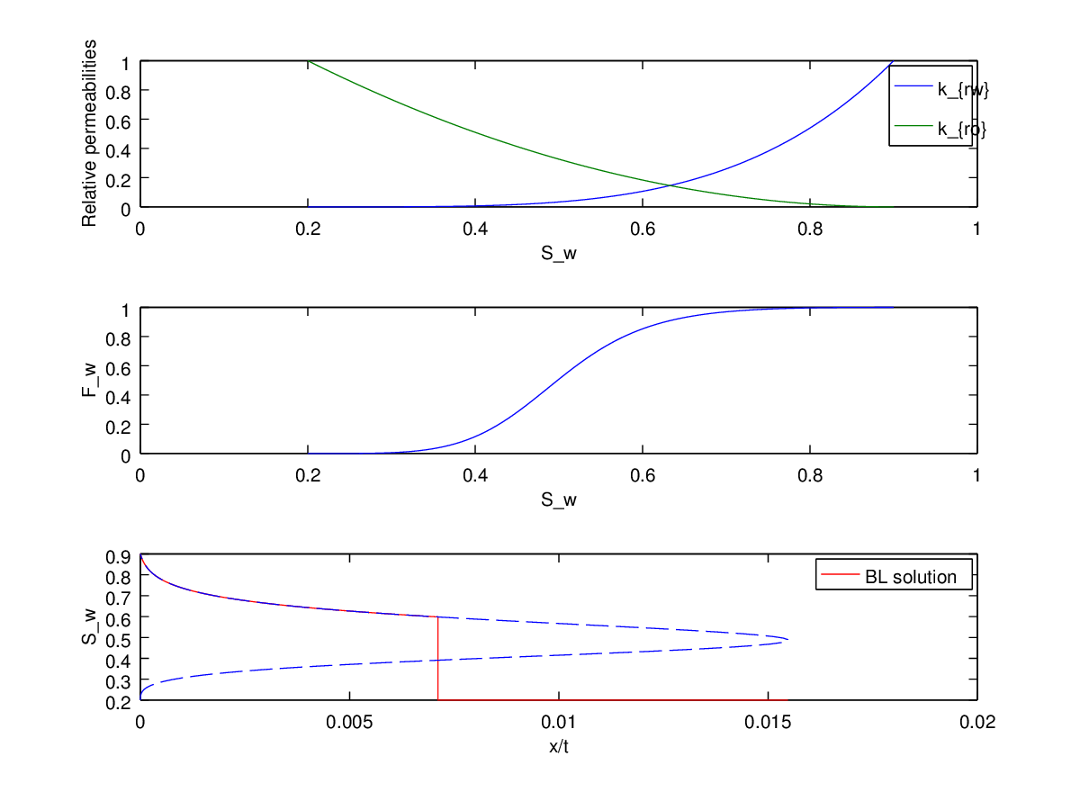
There is an analytical solution for this problem that I know, but I don't quite understand. Let's say the whole domain is initially at $S_{w0}$ and at the left boundary we are injecting with a saturation $S_{w,in}$. We plot $f_w$ versus $S_w$, plot a tangent from the point [$S_{w0}$, $f_w(S_{w0})$] to the curve. This tangent point shows the saturation at the shock front. The rest of the curve from this point to the injection point shows the rarefaction (have no idea what it means) thingy. So from this whole beautiful jiber jaber we derive the following equation at $S_{w,shock}$

$$ \left(\frac{df_w}{dS_w}\right) = \frac{f_w(S_{w0})-f_w(S_{w,shock})}{S_{w0}-S_{w,shock}} $$

that we can solve to find $S_{w,shock}$. Now the story is clear: we move from the injection saturation on the fractional flow curve to the saturation of the shock front and then bang; shock to the initial saturation. The shock moves with a constant speed of $u/\phi$ [m/s].

Optimization and root finding in matlab

In Matlab, we can do the whole thing in a simple script with a lot of @, which I've found out recently that, believe it or not, freaks the hell out of many students! The functions are easy to define:

clc; clear; close all;
% viscosities
muw = 1e-3;
muo = 10e-3;
% initialize the Corey model parameters
kro0 = 1;
krw0 = 1;
no = 2;
nw = 4;
sor = 0.1;
swc = 0.2;
u = 1e-3;
phi = 0.3;
% define the functions
sws = @(sw)((sw-swc)/(1-swc-sor));
dsws = 1/(1-swc-sor);
krw = @(sw)(krw0*sws(sw).^nw);
kro = @(sw)(kro0*(1-sws(sw)).^no);

The above definitions can be used to define the water fractional flow function and then find the shock front saturation. Let's define the fractional flow and its derivative in Matlab:

dkrw = @(sw)(dsws*nw*krw0*sws(sw).^(nw-1));
dkro = @(sw)(-dsws*no*kro0*(1-sws(sw)).^(no-1));
fw = @(sw)((krw(sw)/muw)./(krw(sw)/muw+kro(sw)/muo));
dfw = @(sw)((dkrw(sw)/muw.*kro(sw)/muo-krw(sw)...
/muw.*dkro(sw)/muo)./(krw(sw)/muw+kro(sw)/muo).^2);

The shock front is calculated by solving the nonlinear equation in Matlab in the following way:

% define initial conditions
sw0 = swc; % the reservoir is filled with oil and connate water
% solve the nl equation to find the shock front saturation
sw_shock = fzero(@(sw)(dfw(sw)-(fw(sw0)-fw(sw))./(sw0-sw)), 0.5);

This fzero is a very handy function in Matlab. I use it most of the times and it usually works. It mostly works when, I ask the function to look for the root in a specified range, over which, the function value changes sign. Let's go on and solve the whole thing and plot the result. I explained that the saturation curve moves on the fractional flow curve from the injection point to the shock front and then shocks to the initial condition. I forgot (or didn't, because I write this post at different times) to mention that the main PDE (somewhere above) can be solved by using a method that is called combination of variables (if I remember correctly), and it shows that the front moves with a velocity $(u/\phi) (df_w/dS_w)$. This can be used in the code to plot the water saturation as a function of $x/t$. Now I'm talking nonsense from a very strict mathematical point of view. But if you stay with me, you will see that it works from a practical point of view. The position of each saturation value in space and time is then calculated by

$$ \frac{x}{t} = \frac{u}{\phi} (\frac{dF_w}{dS_w})_{S_w} $$

for $S_w$ between the injection point and shock front. In Matlab, we write it as

% injection saturation
sw_inj = 1-sor; % not to make things too complicated
% water saturation between injection and shock
sw_rf = linspace(sw_inj, sw_shock, 100);
sw_all = linspace(swc, 1-sor, 100); % whole range of possible sw
xt_all = u/phi*dfw(sw_all); % solution over a whole possible range of sw
xt_rf=u/phi*dfw(sw_rf); % rarefaction position
xt_shock = xt_rf(end); % shock front position
plot([xt_rf xt_shock max(xt_all)],...
 [sw_rf sw0 sw0], 'r', xt_all, sw_all, '--b');

This is the final results, generated in octave saved in the following terrible shape due to the lack of a few converters:

The whole script in Matlab/Octave

This is the whole script with a bit more visualization

% A simple compact Matlab/Octave script to solve Buckley-Leverett equation
% for water flooding.
% Written by AAE, TU Delft, September 2014
% Any sort of reproduction and redistribution of this code is highly encouraged.
% Note: The extrapolation of relperm curves is not included to keep
% the code as simple as possible.
clc; clear;
% viscosities
muw = 1e-3;
muo = 10e-3;
% initialize the Corey model parameters
kro0 = 1;
krw0 = 1;
no = 2;
nw = 4;
sor = 0.1;
swc = 0.2;
u = 1e-3;
phi = 0.3;
% define the functions
sws = @(sw)((sw-swc)/(1-swc-sor));
dsws = 1/(1-swc-sor);
krw = @(sw)(krw0*sws(sw).^nw);
kro = @(sw)(kro0*(1-sws(sw)).^no);
% derivatives
dkrw = @(sw)(dsws*nw*krw0*sws(sw).^(nw-1));
dkro = @(sw)(-dsws*no*kro0*(1-sws(sw)).^(no-1));
fw = @(sw)((krw(sw)/muw)./(krw(sw)/muw+kro(sw)/muo));
dfw = @(sw)((dkrw(sw)/muw.*kro(sw)/muo-krw(sw)...
/muw.*dkro(sw)/muo)./(krw(sw)/muw+kro(sw)/muo).^2);
% define initial conditions
sw0 = swc; % the reservoir is filled with oil and connate water
% solve the nl equation to find the shock front saturation
sw_shock = fzero(@(sw)(dfw(sw)-(fw(sw0)-fw(sw))./(sw0-sw)), 0.5);
% injection saturation
sw_inj = 1-sor; % not to make things too complicated
% water saturation between injection and shock
sw_rf = linspace(sw_inj, sw_shock, 100);
sw_all = linspace(swc, 1-sor, 100); % whole range of possible sw
xt_all = u/phi*dfw(sw_all); % solution over a whole possible range of sw
xt_rf=u/phi*dfw(sw_rf);
xt_shock = xt_rf(end);
figure(1);
subplot(3,1,1); plot(sw_all, krw(sw_all), sw_all, kro(sw_all)); 
axis([0 1 0 1]);
xlabel('S_w'); ylabel('Relative permeabilities'); 
legend('k_{rw}', 'k_{ro}');
subplot(3,1,2); plot(sw_all, fw(sw_all)); axis([0 1 0 1]);
xlabel('S_w'); ylabel('F_w');
subplot(3,1,3);plot([xt_rf xt_shock max(xt_all)], ...
[sw_rf sw0 sw0], 'r', xt_all, sw_all, '--b');
xlabel('x/t'); ylabel('S_w'); legend('BL solution');

Next post

the same code in Julia, differences with Matlab