Matlab and Julia -- Part II

In the previous post, I explained how to program the solution procedure of Buckley-Leverett equation in Matlab. Here, I'm trying to move everything to Julia. First, you need to install Julia, and a few important packages. Personally, I prefer the last development version. In Ubuntu-based distributions, you can install it by writing the following lines in the terminal.

sudo add-apt-repository ppa:staticfloat/julianightlies
sudo add-apt-repository ppa:staticfloat/julia-deps
sudo apt-get update
sudo apt-get install julia

You can get installers for other OS's here.
First, install a few dependencies, including python 2.7 and matplotlib. Then, run Julia and add the PyPlot and Roots packages, by typing

Pkg.add("Roots")
Pkg.add("PyPlot")

Now, you can proceed to the next step, writing the code in Julia. There are a few things that you need to now when you start working with Julia as a Matlab user. In Matlab, you write

a=linspace(0,1,100);
b=1;
c=rand(size(a));
a(1) % 0
a(end) % 1
length(a) % 100
size(a) % 1   100
size(b) % 1   1
b*a
a.*c

and in Julia, you write

a=linspace(0,1,100)
b=1
c=rand(size(a))
a[1]
a[end]
length(a)  # 100
size(a)    # (100,)
size(b)   # ()
b*a
a.*c

In Matlab, all the variables are 2D matrices. In Julia, they are not. Now try to get used to it. For me, it was the hardest part, next to the fact that there is not a good IDE for Julia yet.
No I convert everything right away to Julia, and you can compare it to the Matlab code for yourself.

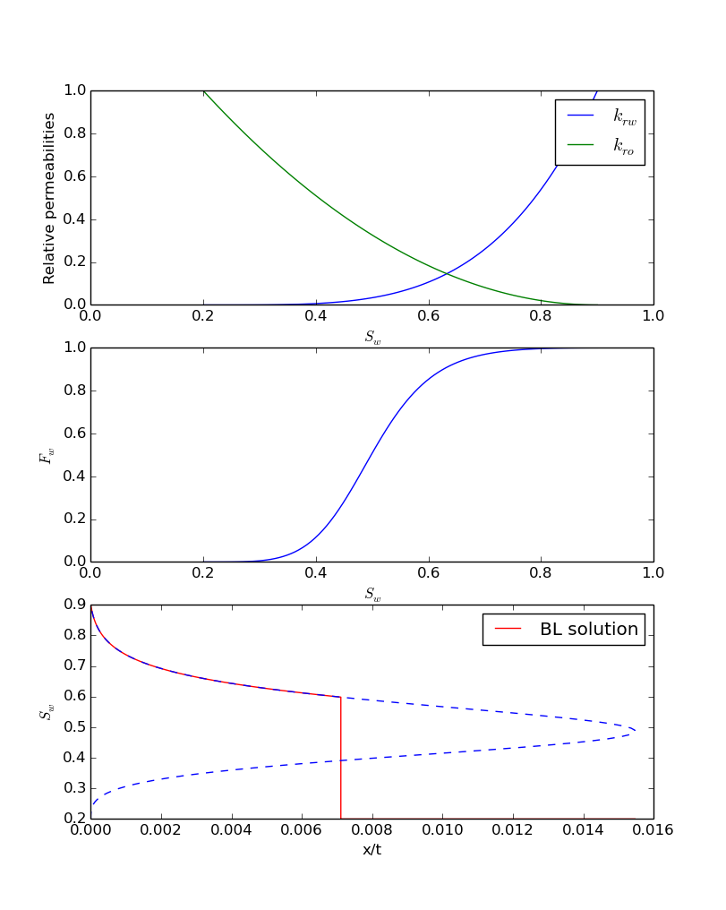
# A simple compact Julia script to solve Buckley-Leverett equation
# for water flooding.
# Written by AAE, TU Delft, September 2014
# Any sort of reproduction and redistribution of this code is highly encouraged.
# Note: The extrapolation of relperm curves is not included to keep
# the code as simple as possible.
# run the following two lines first:
# using Roots
# using PyPlot
# viscosities
muw = 1e-3
muo = 10e-3
# initialize the Corey model parameters
kro0 = 1
krw0 = 1
no = 2
nw = 4
sor = 0.1
swc = 0.2
u = 1e-3
phi = 0.3
# define the functions
sws(sw)=((sw-swc)/(1-swc-sor))
dsws = 1/(1-swc-sor)
krw(sw)=(krw0*sws(sw).^nw)
kro(sw)=(kro0*(1-sws(sw)).^no)
# derivatives
dkrw(sw)=(dsws*nw*krw0*sws(sw).^(nw-1))
dkro(sw)=(-dsws*no*kro0*(1-sws(sw)).^(no-1))
fw(sw)=((krw(sw)/muw)./(krw(sw)/muw+kro(sw)/muo))
dfw(sw)=((dkrw(sw)/muw.*kro(sw)/muo-krw(sw)/muw.*dkro(sw)/muo)./(krw(sw)/muw+kro(sw)/muo).^2)
# define initial conditions
sw0 = swc # the reservoir is filled with oil and connate water
# solve the nl equation to find the shock front saturation
f_shock(sw)=(dfw(sw)-(fw(sw0)-fw(sw))./(sw0-sw))
sw_shock = fzero(f_shock, 0.5)
# injection saturation
sw_inj = 1-sor  # not to make things too complicated
# water saturation between injection and shock
sw_rf = linspace(sw_inj, sw_shock, 100)
sw_all = linspace(swc, 1-sor, 100) # whole range of possible sw
xt_all = u/phi*dfw(sw_all) # solution over a whole possible range of sw
xt_rf=u/phi*dfw(sw_rf)
xt_shock = xt_rf[end]
figure(1)
subplot(3,1,1) 
plot(sw_all, krw(sw_all), sw_all, kro(sw_all)) 
axis([0, 1, 0, 1])
xlabel(L"S_w") 
ylabel("Relative permeabilities") 
legend((L"k_{rw}", L"k_{ro}"))
subplot(3,1,2) 
plot(sw_all, fw(sw_all))
axis([0, 1, 0, 1])
xlabel(L"S_w") 
ylabel(L"F_w")
subplot(3,1,3)
plot([xt_rf, xt_shock, maximum(xt_all)], [sw_rf, sw0, sw0], "r", xt_all, sw_all, "--b")
xlabel("x/t") 
ylabel(L"S_w") 
legend(("BL solution",))

Now is the important step, running the code. Load the packages that you are going to call from your code:

using Roots
using PyPlot

We will use fzero function from Roots package to find the shock front. We will also use the PyPlot package to visualize the results. Now load the code in Julia by typing

reload("BLjulia.jl")

If everything is fine, it will show you the following plot:

I'll discuss some of the small issues that I had with Julia as a Matlab user.